
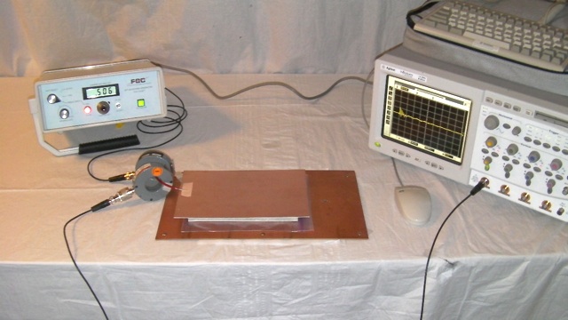
Figure 1. Test Setup For Measuring The Resonance of Two PCBs Connected by a Wire
Abstract: Current probes can
be used to inductively couple voltage pulses into cables for
troubleshooting without needing a direct
connection to the circuit. Using this method, data is presented to characterize the
resonance of two circuit boards connected by a wire and some factors
that affect the resonance.
Discussion: Figure 1 shows the
test setup used for this Technical Tidbit. The setup is composed of two copper clad boards connected by a wire about
four inches (~10 cm) long, a Fischer TG-EFT pulse generator, two
current probes, and a scope. The two boards are separated about an inch
(~2.5 cm) by a paperback book. One current probe, a Fischer F-62b, was used to inject pulses and the other, a Fischer F-65, was used to monitor the current.
A Fischer Custom Communications TG-EFT high voltage pulse generator was used to drive the F-62b current probe. The TG-EFT output has a fast risetime of about 2 nanoseconds and a slow fall time of several tens of nanoseconds. Since the F-62b has a low frequency cutoff well above 100 MHz, only the higher frequency components of the TG-EFT are injected. This characteristic of the F-62b is not necessary for many investigations but can be useful as well.
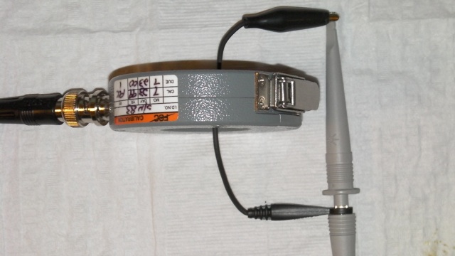
Figure 2 shows the F-62b clamped around the ground wire shorting an Agilent 1163a 500 Ohm resistive one GHz probe. The 500 Ohm input resistance of the probe is high enough so that the probe measures the open circuit voltage that the F-62b injects into circuits. The result is shown in Figure 3.
In Figure 3, one can see a peak voltage of about 8 volts (for a TG-EFT setting of about 500 Volts open circuit). Figure 4 shows the signal expanded from 20 ns/div to 5 ns/div. The smaller peaks after the initial one are reflections off the series 50 Ohm termination I was using with the TG-EFT generator.
Figure 4. Open Circuit Voltage Induced in the Agilent 1163A Probe
(Vertical scale = 2 Volts/div, Horizontal scale = 5 ns/div)
Figure 5 shows the two current probes attached to the wire connecting the copper clad boards and Figure 6 shows the resulting waveform measured by the F-65 current probe.
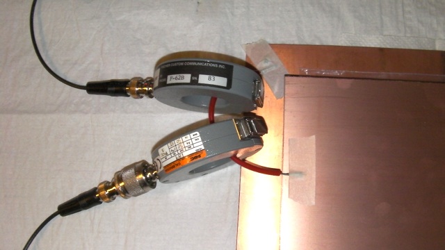
Figure 5. Close-up Showing Two Current Probes on the Wire Connecting the Copper Clad Boards
A damped sinusoid is clearly seen with an amplitude of about 400 mA peak (the F-65 has a one Ohm or one Volt/Amp transfer impedance). Figure 7 expands the waveform from 100 ns/div out to 20 ns/div where the oscillating frequency is seen to be about 77 MHz. The capacitance of the two copper clad boards together with the inductance of the wire connecting them results in a fairly high Q resonant circuit at 77 MHz. I have seen structures like this in many electronic products and such structures can result in operational problems or failures of EMC tests.
Figure 7. Current Measured Between Two Copper Clad Boards
(Vertical scale = 100 mA/div, Horizontal scale = 20 ns/div)
Figure 8 shows the paperback book removed from between the copper clad boards and replaced with a plastic bag so the spacing is now around 1 mm instead of a few cm. Figure 9 shows the result and Figure 10 expands the time scale from 50 ns/div to 20 ns/div.
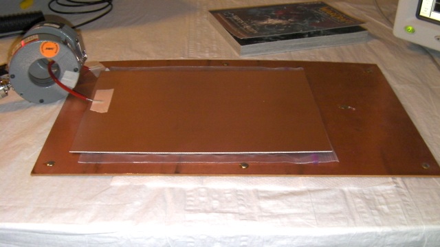
Figure 8. Copper Clad Boards Separated by Plastic Bag
Figure 9. Current Measured Between Two Copper Clad Boards at 1 mm Spacing
(Vertical scale = 200 mA/div, Horizontal scale = 50 ns/div)
Figure 10. Current Measured Between Two Copper Clad Boards at 1 mm Spacing
(Vertical scale = 200 mA/div, Horizontal scale = 20 ns/div)
The waveforms in Figures 9 and 10 are different in two main ways from the waveforms in Figures 6 and 7. First the frequency of oscillation is lower, now about 34 MHz instead of 77 MHz. In addition the amplitude has increased to nearly 600 mA, up from a little over 400 mA. These effects are related to the increased capacitance between the boards.
Resonance measurements such as those above can be made with magnetic loop probes, but the use of current probes can give a wider bandwidth, greater amplitude of the output signal, and a more repeatable measurement.
A Fischer Custom Communications TG-EFT high voltage pulse generator was used to drive the F-62b current probe. The TG-EFT output has a fast risetime of about 2 nanoseconds and a slow fall time of several tens of nanoseconds. Since the F-62b has a low frequency cutoff well above 100 MHz, only the higher frequency components of the TG-EFT are injected. This characteristic of the F-62b is not necessary for many investigations but can be useful as well.
Figure 2 shows the F-62b clamped around the ground wire shorting an Agilent 1163a 500 Ohm resistive one GHz probe. The 500 Ohm input resistance of the probe is high enough so that the probe measures the open circuit voltage that the F-62b injects into circuits. The result is shown in Figure 3.
Figure 2. Measuring the Open Circuit Voltage Injected by the F-62b Current Probe
Figure 3. Open Circuit Voltage Induced in the Agilent 1163A Probe
(Vertical scale = 2 Volts/div, Horizontal scale = 20 ns/div)
(Vertical scale = 2 Volts/div, Horizontal scale = 20 ns/div)
In Figure 3, one can see a peak voltage of about 8 volts (for a TG-EFT setting of about 500 Volts open circuit). Figure 4 shows the signal expanded from 20 ns/div to 5 ns/div. The smaller peaks after the initial one are reflections off the series 50 Ohm termination I was using with the TG-EFT generator.
Figure 4. Open Circuit Voltage Induced in the Agilent 1163A Probe
(Vertical scale = 2 Volts/div, Horizontal scale = 5 ns/div)
Figure 5 shows the two current probes attached to the wire connecting the copper clad boards and Figure 6 shows the resulting waveform measured by the F-65 current probe.
Figure 5. Close-up Showing Two Current Probes on the Wire Connecting the Copper Clad Boards
Figure 6. Current Measured Between Two Copper Clad Boards
(Vertical scale = 100 mA/div, Horizontal scale = 100 ns/div)
(Vertical scale = 100 mA/div, Horizontal scale = 100 ns/div)
A damped sinusoid is clearly seen with an amplitude of about 400 mA peak (the F-65 has a one Ohm or one Volt/Amp transfer impedance). Figure 7 expands the waveform from 100 ns/div out to 20 ns/div where the oscillating frequency is seen to be about 77 MHz. The capacitance of the two copper clad boards together with the inductance of the wire connecting them results in a fairly high Q resonant circuit at 77 MHz. I have seen structures like this in many electronic products and such structures can result in operational problems or failures of EMC tests.
Figure 7. Current Measured Between Two Copper Clad Boards
(Vertical scale = 100 mA/div, Horizontal scale = 20 ns/div)
Figure 8 shows the paperback book removed from between the copper clad boards and replaced with a plastic bag so the spacing is now around 1 mm instead of a few cm. Figure 9 shows the result and Figure 10 expands the time scale from 50 ns/div to 20 ns/div.
Figure 8. Copper Clad Boards Separated by Plastic Bag
Figure 9. Current Measured Between Two Copper Clad Boards at 1 mm Spacing
(Vertical scale = 200 mA/div, Horizontal scale = 50 ns/div)
Figure 10. Current Measured Between Two Copper Clad Boards at 1 mm Spacing
(Vertical scale = 200 mA/div, Horizontal scale = 20 ns/div)
The waveforms in Figures 9 and 10 are different in two main ways from the waveforms in Figures 6 and 7. First the frequency of oscillation is lower, now about 34 MHz instead of 77 MHz. In addition the amplitude has increased to nearly 600 mA, up from a little over 400 mA. These effects are related to the increased capacitance between the boards.
Resonance measurements such as those above can be made with magnetic loop probes, but the use of current probes can give a wider bandwidth, greater amplitude of the output signal, and a more repeatable measurement.
Summary:
Current probes can be used to induce series voltage impulses in cables.
In this case, the series voltage pulses were used to investigate the
resonance between two copper clad boards and the effects of board
spacing. Resonance between two boards, as illustrated here, can cause
system operational problems and issues with EMC compliance in some cases.
Additional articles on this website related to this topic are:
- Current Probes, More Useful
Than You Think (~170K)
(1998 IEEE EMC Symposium paper) - January 2006, A Small Change Can Have a Large Effect
- October 2007, Using Noise Injection for Troubleshooting Circuits
- November 2007, Measuring Structural Resonances in the Time Domain - Part 1
- December 2007, Using Current Probes to Inject Pulses for Troubleshooting
(Current Probes, More Useful Than You Think - Part 2) - March 2009, Using Current Probes to Inject Pulses for Troubleshooting - Part 2
(Current Probes, More Useful Than You Think - Part 3) - April 2009, Construction of a Series 50 Ohm Termination
- May 2009, Using a Series 50 Ohm Termination With a High Voltage Transient Generator
- The scope used in this Technical Tidbit is an Agilent Infinium 54845a scope
- The Agilent 1163a probe is a 10:1 resistive divider probe with over 1 GHz bandwidth.
- Fischer Custom Communications F-62b and F-65 current probes
- Fischer Custom Communications TG-EFT high voltage pulse generator
Click here for a description of my latest seminar titled (now also available online as a WebEx seminar):
EMC
Lab Techniques for Designers
(How to find EMC problems and have some confidence your system will pass EMC testing while it is still in your lab).
(How to find EMC problems and have some confidence your system will pass EMC testing while it is still in your lab).
 |
Check
out my podcast containing mp3 format short tutorials, tech news and
more! Just click on the
microphone to see the listing
of free
audio programs. Content is added every week on technical
topics so check back frequently. |
Home